Lucas-Kanade Tracking
In this assignment, I implemented 2 different variants of the famous Lucas-Kanade Tracking algorithm.
Lucas-Kanade Tracking
In the first variant, we implemented a simple Lucas & Kanade tracker with one single template. In the scenario of two-dimensional tracking with a pure translation warp function,
\[W(x;p) = x + p\]The problem can be described as follows: starting with a rectangular neighborhood of pixels \(\mathbb{N} \in \{ \bf {x_d} \}^{D}_{d=1}\) on frame \(I_t\), the Lucas-Kanade tracker aims to move it by an offset \(\mathbf{p} = [ p_x, p_y ]^T\) to obtain another rectangle on frame \(I_{t+1}\), so that the pixel squared difference in the two rectangles is minimized:
\[\mathbf{p^*} = argmin_{\mathbf{p}} \sum_{\mathbf{x} \in \mathbb{N}} || I_{t+1}(\mathbf{x + p}) - I_{t}(\mathbf{x})||_{2}^{2}\]Running the simple KLT gives us the following output:
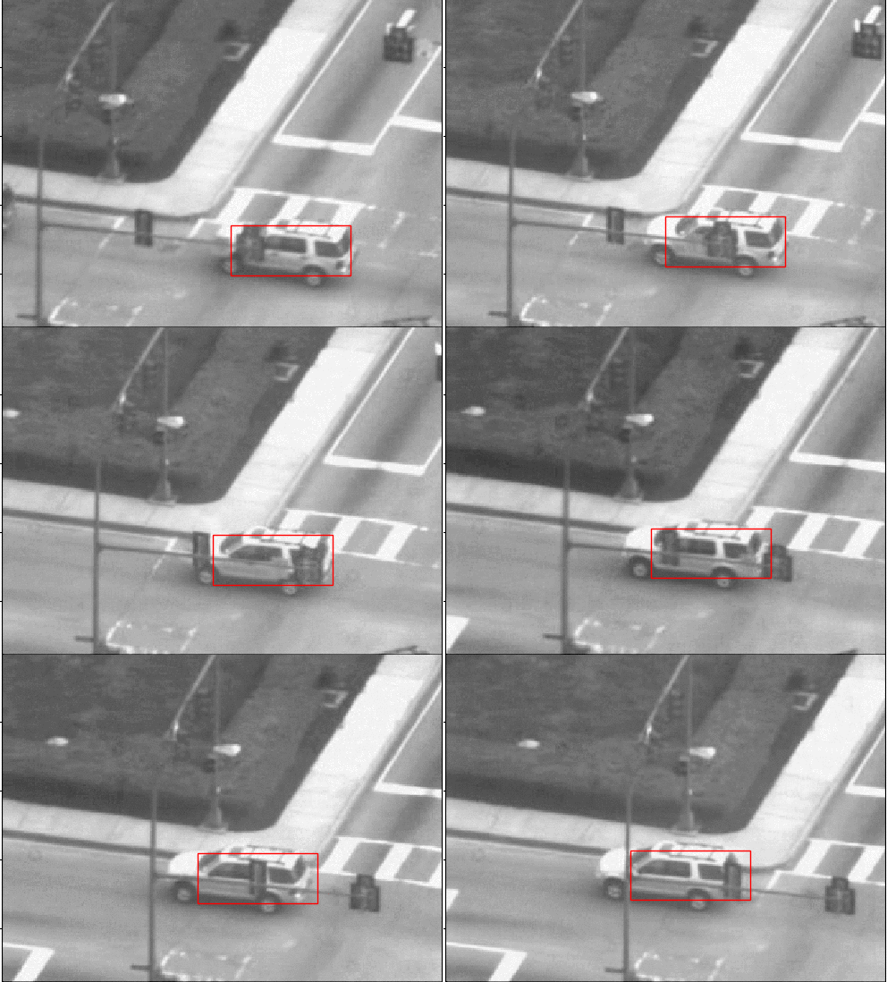
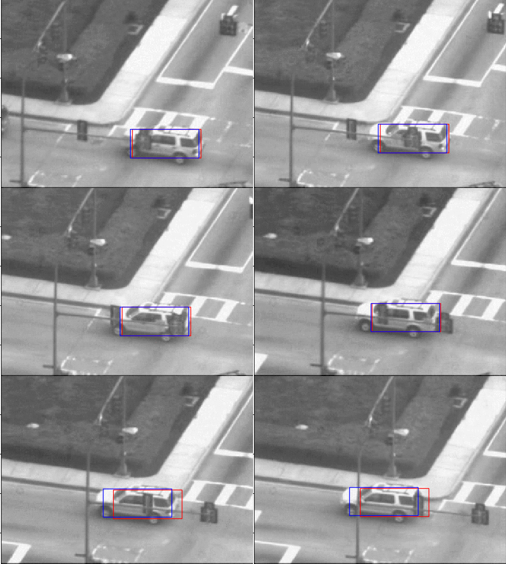
We can see that the car we are tracking differs in appearance from the first and the last frame. Along with this, we are also updating the template after processing each frame and the error is accumulating whihc is lead to a drift in the template. We us [1] to help solve the problem and the updated tracking can be seen the below footage with a blue bounding box.
Affine Motion Subtraction
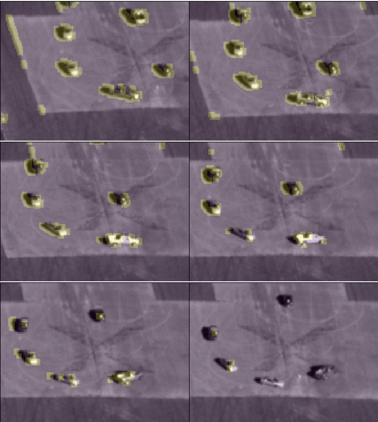
In the above section we assumed the the motion is limited to pure translation, in this section we implemented a tracker for estimating dominant affine motion in a sequence of images and subsequently identify pixels corresponding to moving objects in the scene.
To estimate dominant motion, the entire image \(I_{t}\) serves as the template to be tracked in image \(I_{t+1}\), that is, \(I_{t+1}\) is assumed to be approximately an affine warped version of \(I_{t}\). This approach is reasonable under the assumption that a majority of the pixels correspond to the stationary objects in the scene whose depth variation is small relative to their distance from the camera.
Using a planar affine warp function you can recover the vector \(\Delta p = [ p^1 , . . . , p^6 ]^{T}\),
\(\mathbf{x'} = \mathcal{W}(\mathbf{x;p}) = \begin{bmatrix} 1 + p_{1} & p_{2} \\ p_{4} & 1 + p_{1} \end{bmatrix} \begin{bmatrix} x \\ y \end{bmatrix} + \begin{bmatrix} p_{3} \\ p_{6} \end{bmatrix}\).
One can represent this affine warp in homogeneous coordinates as,
\[\widetilde{\mathbf{x}}' = \mathbf{M} \widetilde{\mathbf{x}}\]where,
\[M = \begin{bmatrix} 1 + p_{1} & p_{2} & p_{3} \\ p_{4} & 1 + p_{5} & p_{6} \\ 0 & 0 & 1 \end{bmatrix}\]Once we are able to compute the transformation matrix \mathbf{M} relating an image pair \(I_{t}\) and \(I_{t+1}\), a naive way for determining pixels lying on moving objects is as follows: warp the image It using \mathbf{M} so that it is registered to \(I_{t+1}\) and subtract it from \(I_{t+1}\) ; the locations where the absolute difference exceeds a threshold can then be declared as corresponding to locations of moving objects. We can visualise the results below: